Results for D⁰- D⁰ Mixing

(assuming CP conservation)

For a complete list of references click here

For mixing results allowing for CP violation click here

Notation: the mass eigenstates are denoted D ₁ ≡ p|D⁰> + q|D⁰> and D ₂ ≡ p|D⁰> − q|D⁰>; R _D is the ratio of magnitudes of D⁰ → f and D⁰ → f amplitudes; and δ (φ) is the strong (weak) phase difference between D⁰ → f and D⁰ → f amplitudes.

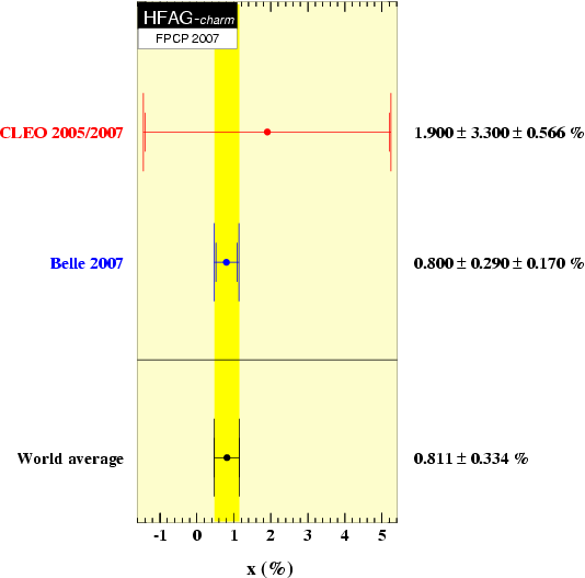
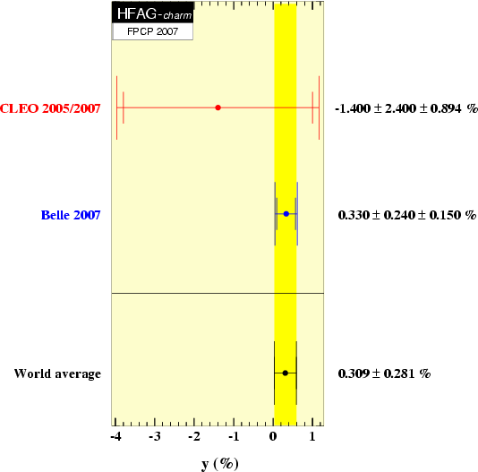
This page is organized as follows. First, "pure" measurements and their world averages are presented:

• D⁰ → K⁺l⁻ ν :   constraint on R _M ≡ (x²+y²)/2     (here)
• D⁰ → K⁺ K⁻, π⁺ π⁻ :   constraints on y _CP = (1/2)(|q/p| + |p/q|) y cosφ − (1/2)(|q/p| − |p/q|) x sin φ, and
                                              A _Γ = (1/2)(|q/p|−|p/q|) y cosφ −(1/2)(|q/p|+|p/q|) x sin φ     (here)
• D⁰ → K⁺ π ⁻ :   constraints on R _D, x' ≡ x cosδ + y sin δ, and y' ≡ y cosδ - x sin δ     (here)
• D⁰ → K⁺ π ⁻ π ⁰ and K⁺ π ⁻ π ⁺ π ⁻ :   constraints on R _B, R _M, <R _D>, and α<y'>     (here)
• D⁰ → K⁰_S π⁺ π ⁻ :   constraints on x and y     (here)
• Ψ(3770) → D⁰-D⁰ reactions :   constraints on R _M, y, and δ     (here)

• combined result for R _M   (all data)     (here)
• combined result for y   (all data)     (here)
• combined results for x, y, and δ   (all data)     (here)
  The final results for no CPV are:     x = (0.87 ^+0.30 _−0.34 )%,     y = (0.66 ^+0.21 _−0.20 )%,     δ = (0.33 ^+0.26 _−0.29 ) radians.

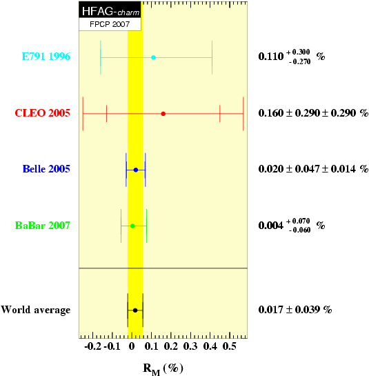
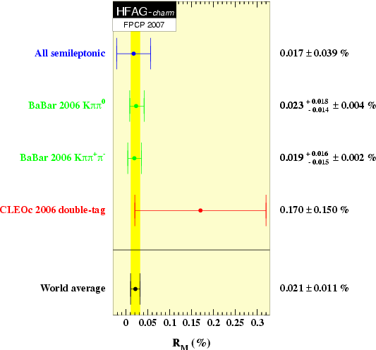
D⁰ → K⁺l⁻ ν results for R _M ≡ (x²+y²)/2.

Year	Experiment	Result	Comment
1996	FNAL E791	R M = (0.11 +0.30 −0.27 +0.00 −0.014 )%	500 GeV π −N interactions (2 × 1010 events)
2005	CLEO II.V	R M = (0.16 ± 0.29 ± 0.29 )%	9.0 fb−1 near Υ(4S) resonance
2004	BaBar	R M = (0.23 ± 0.12 ± 0.04 )%	87 fb−1 near Υ(4S) resonance
2005	Belle	R M = (0.020 ± 0.047 ± 0.014 )%	253 fb−1 near Υ(4S) resonance
2007	BaBar	R M = (0.004 +0.070 −0.060 )%	344 fb−1 near Υ(4S) resonance; decays are "double-tagged" (tag side is fully reconstructed)
	COMBOS average	R M = (0.0173 ± 0.0387 )% CL = 0.965	(output)   stat. and syst. errors assumed uncorrelated; BaBar 2004 result not included as correlation with BaBar 2007 not yet determined

            Plot of average:

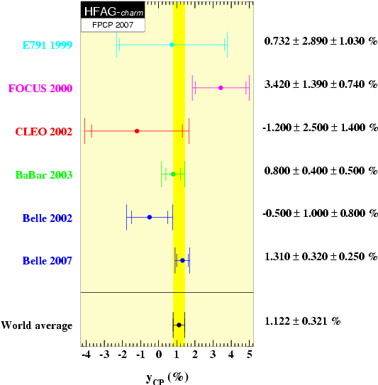
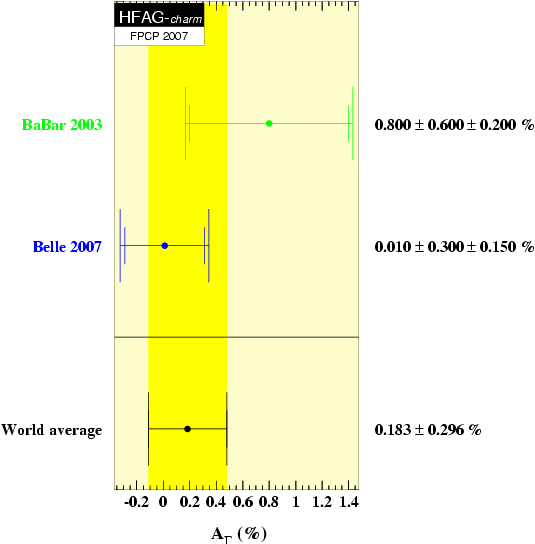
D⁰ → K⁺ K⁻, π⁺ π⁻ results for: y _CP ≡ [Γ(CP+)/<Γ>]−1 = (1/2)(|q/p| + |p/q|) y cosφ − (1/2)(|q/p| − |p/q|) x sin φ, and A _Γ ≡ [τ(D⁰ → K⁺ K⁻) − τ(D⁰ → K⁺ K⁻ )] / [τ(D⁰ → K⁺ K⁻) + τ(D⁰ → K⁺ K⁻ )] = (1/2)(|q/p|−|p/q|) y cosφ −(1/2)(|q/p|+|p/q|) x sin φ .

Year	Experiment	Result	Comment
1999	FNAL E791	ΔΓ = (0.04 ± 0.14 ± 0.05 ) ps −1	500 GeV π −N interactions (2 × 1010 events)
2000	FOCUS	y CP = (3.42 ± 1.39 ± 0.74 )%	γN interactions (1 × 106 reconstr. D → K n(π) decays)
2002	CLEO II.V	y CP = (−1.2 ± 2.5 ± 1.4 )%	9.0 fb−1 near Υ(4S) resonance
2003	BaBar	y CP = (0.8 ± 0.4 +0.5 −0.4 )% A Γ = (0.8 ± 0.6 ± 0.2 )%	91 fb−1 near Υ(4S) resonance
2002	Belle	y CP = (−0.5 ± 1.0 +0.7 −0.8 )%	23.4 fb−1 near Υ(4S) resonance; no D* tag
2007	Belle	y CP = (1.31 ± 0.32 ± 0.25 )% A Γ = (0.01 ± 0.30 ± 0.15 )%	540 fb−1 near Υ(4S) resonance
	COMBOS average	y CP = (1.12 ± 0.32 )% CL = 0.430 A Γ = (0.18 ± 0.30 )% CL = 0.270	( output for y CP )   ( output for A Γ ) symmetrized statistical, systematic errors; stat. errors for two Belle analyses have correl.= 0.0165; all systematic errors assumed uncorrelated

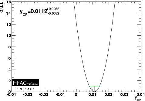
            Plot of y _CP average:                                                                   Plot of A _Γ average:

            Likelihood function: [LF #1]

D⁰ → K⁺ π ⁻ results for R _D, x' ≡ x cosδ + y sin δ, y' ≡ y cosδ - x sin δ, and R _B ≡ R _D + y' √ R _D + (x²+y²)/2 . These results assume no CPV.

Year	Experiment	Result	Comment
1998	FNAL E791	RB = (0.68 +0.34 −0.33 ± 0.07)%	500 GeV π −N interactions (2 × 1010 events)
2000	CLEO II.V	RB = (0.332 +0.063 −0.065 ± 0.040)% RD = (0.47 +0.11 −0.12 ± 0.04)% x' = (0.0 ± 1.5 ± 0.2)% y' = (− 2.3 +1.3 −1.4 ± 0.3)%	9.0 fb−1 near Υ(4S) resonance
2005	FOCUS	RB = (0.429 +0.063 − 0.061 ± 0.027)% RD = (0.381 +0.167 − 0.163 ± 0.092)% x' 2 = − 0.059% y' = 1.0%	γN interactions (1 × 106 reconstr. D → K n(π) decays)
2006	Belle	RB = (0.377 ± 0.008 ± 0.005)% RD = (0.364 ± 0.017)% x' 2 = (0.018 +0.021 −0.023 )% y' = (0.06 +0.40 −0.39 )%	400 fb−1 near Υ(4S) resonance
2006	CDF (Run II)	RB = (0.405 ± 0.021 ± 0.011)%	0.35 fb−1 at √s = 1.96 TeV
2007	BaBar	RD = (0.303 ± 0.016 ± 0.010)% x' 2 = (−0.022 ± 0.030 ± 0.021)% y' = (0.97 ± 0.44 ± 0.31)%	384 fb−1 near Υ(4S) resonance

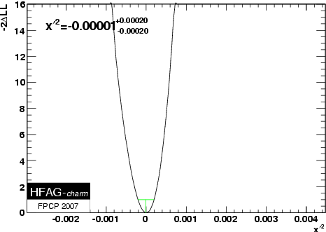
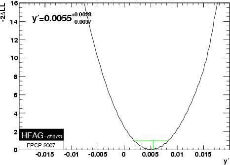
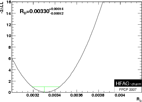
To combine K⁺ π ⁻ results, the three-dimensional log(likelihood) functions for (x'², y', R_D) are added (Belle + BaBar only) . The resulting function is mapped onto the (x'², y') plane as follows: for a specific (x'², y') value, the parameter R_D is allowed to seek its preferred value, and the resulting likelihood is assigned. The function is mapped onto the R_D axis as follows: for a specific R_D value, the parameters x'² and y' are allowed to seek their preferred values, and the resulting likelihood is assigned.

To map the (x'², y') likelihood function to an (x, y, δ) likelihood volume, the (x, y, δ) space is scanned and, at each point, (x'², y') is calculated and the corresponding likelihood assigned. Note that this likelihood value must come from the physical region of the (x'², y') plane, i.e., positive x'².

To map the (x, y, δ) likelihood volume onto the (x, y) plane, the (x, y) space is scanned and, at each point, the parameter δ is allowed to seek its preferred value, and the corresponding likelihood is assigned.

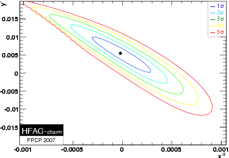
      Belle + BaBar (x'², y') projection:                                           x'² projection:

                       

      y' projection:                                                                         R_D projection:

                       

      (x'², y') → (x, y) mapped likelihood [LF #2] :

         

D⁰ → K⁺ π ⁻ π ⁰ and K⁺ π ⁻ π ⁺ π ⁻ results for R _B, R _M, <R _D>, and α<y'>, where <…> denotes a quantity integrated (or averaged) over the selected phase-space region of the Dalitz plot, and α is a suppression factor in the range (0,1) arising from strong phase differences over the Dalitz plot. These results assume no CPV.

Year	Experiment	Result	Comment
2005	Belle	RB(K + π − π 0) = (0.229 ± 0.015 +0.013 −0.009 )% RB(K + π − π + π− ) = (0.320 ± 0.018 +0.018 −0.013 )%	281 fb−1 near Υ(4S) resonance
2006	BaBar	RB(K + π − π 0) = (0.214 ± 0.008 ± 0.008)% RM = (0.023 +0.018 −0.014 ± 0.004)% <RD(K + π − π 0) > = (0.164 +0.026 −0.022 ± 0.012)% α<y'(K + π − π 0) > = (−0.012 +0.006 −0.008 ± 0.002)%	230.4 fb−1 near Υ(4S) resonance
2006	BaBar	RM = (0.019 +0.016 −0.015 ± 0.002)% α<y'(K + π − π+ π−)> = (− 0.6 ± 0.5 ± 0.1)%	230.4 fb−1 near Υ(4S) resonance

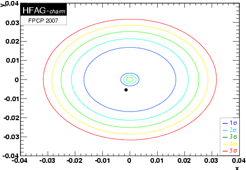
D⁰ → K⁰_S π⁺ π ⁻ results. These results assume no CPV.

Year	Experiment	Result	Comment
2005/2007	CLEO II.V	x = (1.9 +3.2 −3.3 ± 0.4 ± 0.4)% y = (−1.4 ± 2.4 ± 0.8 ± 0.4)%	9.0 fb−1 near Υ(4S) resonance; The errors are statistical, experimental systematic, and decay model systematic, respectively.
2007	Belle	x = (0.80 ± 0.29 ± 0.17)% y = (0.33 ± 0.24 ± 0.15)%	540 fb−1 near Υ(4S) resonance
	COMBOS average	x = (0.811 ± 0.334 )%   CL = 0.74 y = (0.309 ± 0.281 )%   CL = 0.50	(output for x)   (output for y) symmetrized statistical, systematic errors; stat. and syst. errors assumed uncorrelated

            Plot of x average:                                                                                     Plot of y average:

            Likelihood function in (x, y) plane [LF #3] :

Ψ(3770) → D⁰-D⁰ results, using correlations. The errors are statistical only.

Year	Experiment	Result	Comment
2006	CLEO-c	RM = (0.17 ± 0.15)% y = (−5.8 ± 6.6)% cos δK π = 1.09 ± 0.66	0.281 fb−1 at Ψ(3770) resonance

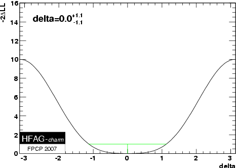
            Likelihood function for δ [LF #4] :

R _M combination:

Year	Measurement	Result	Comment
	All D0 → K+l− ν	R M = (0.017 ± 0.039 )% CL = 0.965	(output)   stat. and syst. errors assumed uncorrelated
2006	BaBar D0 → K+ π π	RM = (0.023 +0.018 −0.014 ± 0.004)%	230.4 fb−1 near Υ(4S) resonance
2006	BaBar D0 → K+ π π π	RM = (0.019 +0.016 −0.015 ± 0.002)%	230.4 fb−1 near Υ(4S) resonance
2006	CLEO-c	RM = (0.17 ± 0.15)%	0.281 fb−1 at Ψ(3770) resonance
	COMBOS average	R M = (0.021 ± 0.011 )% CL = 0.795	(output)   stat. and syst. errors assumed uncorrelated

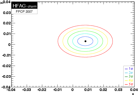
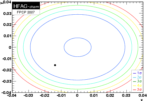
            Plot of overall average:                                                                         Likelihood function in (x, y) plane [LF #5] :

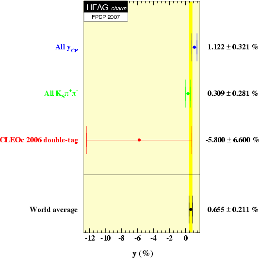
y combination assuming y _CP =y, and that y from D⁰ → K_S π⁺ π ^- corresponds to [Γ(CP+)−Γ(CP−)]/(2Γ).

Year	Measurement	Result	Comment
	All yCP	y CP = (1.12 ± 0.32 )% CL = 0.430	(output)   stat. and syst. errors assumed uncorrelated
	All D0 → KS π+ π -	y = (0.309 ± 0.281 )% CL = 0.50	(output) symmetrized statistical, systematic errors; stat. and syst. errors assumed uncorrelated
2006	CLEO-c	y = (-5.8 ± 6.6)%	0.281 fb−1 at Ψ(3770) resonance
	COMBOS average	y = (0.655 ± 0.211 )% CL = 0.101	(output)   stat. and syst. errors assumed uncorrelated

            Plot of overall average:

Combination of all data assuming no CP violation (y _CP =y) and that y from D⁰ → K_S π⁺ π ^- corresponds to [Γ(CP+)−Γ(CP−)]/(2Γ).

To combine all results, we convert each measurement to a likelihood function in (x, y, δ) space and sum the log(likelihoods). The input likelihood functions are shown above: LF #1, LF #2, LF #3, LF #4, LF #5.

The resulting (x, y, δ) likelihood function is mapped to the (x, y) plane as follows: for a specific (x, y) value, the parameter δ is allowed to seek its preferred value, and the corresponding likelihood is assigned.

To map the likelihood function to the x axis: for a specific x value, the parameters y and δ are allowed to seek their preferred values, and the corresponding likelihood is assigned.

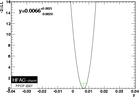
To map the likelihood function to the y axis: for a specific y value, the parameters δ and x are allowed to seek their preferred values, and the corresponding likelihood is assigned.

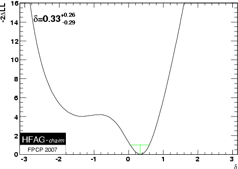
To map the likelihood function to the δ axis: for a specific δ value, the parameters x and y are allowed to seek their preferred values, and the corresponding likelihood is assigned.

            Overall likelihood function in (x, y) plane:                                     Overall likelihood function for δ :

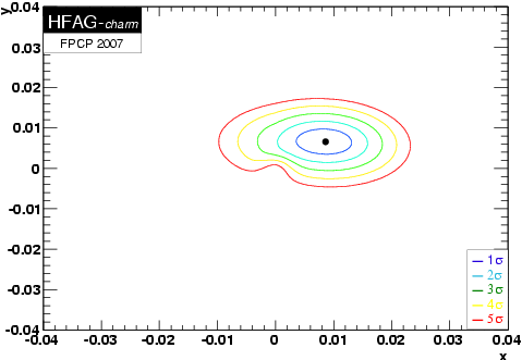
            Overall likelihood function for x:                                                 Overall likelihood function for y: